Published:2026-10-19 12:00:00
Updated:
Linear actuators · Motion and timing
A move is useful when the next operation can begin
A carriage advances 50 mm, stops and returns. That simple action contains acceleration, settling, inspection and waiting. Separating those intervals gives design and commissioning teams a shared language and a practical place to start improving the cycle.
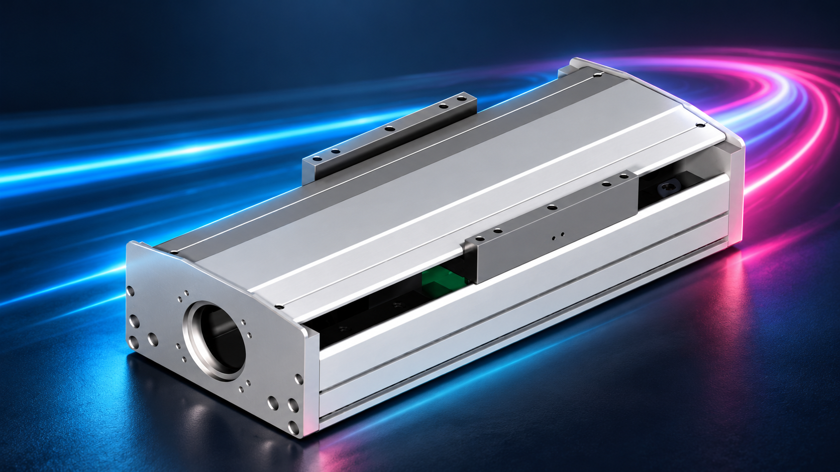
01 / Complete cycle
Define how one part completes its task
Consider an inspection station: the carriage advances, the workpiece settles, the camera takes an image and the carriage returns. The end of the motion command is not necessarily the start of a usable exposure. Writing down the sequence shows which interval is worth improving.
Tcycle = Σtmove + Σtsettle + Σtprocess + Σtwait
For sequential, non-overlapping stages; all times are in seconds.| Interval | Definition used here | What to record |
|---|---|---|
| Move | Start to end of the planned trajectory, including acceleration, cruise and deceleration. | Controller trajectory timestamps and feedback on a shared timebase. |
| Settle | Additional time after the planned move until the process error criterion is met for its required duration. | Measurement point, error band and qualifying duration. |
| Process | Clamping, imaging, dispensing or inspection activity. | Whether it needs a stable position and what the completion signal means. |
| Wait | Non-overlapping handshakes, infeed, interlocks and other delays. | Sequence logs; avoid counting time already included in another stage. |
For parallel axes or overlapping processes, follow the actual critical path. Do not simply add every axis time. State parts per cycle and any upstream or downstream constraints.
02 / Move duration
The speed limit may never be reached
Use a simple model that is easy to audit: zero start and finish speed, equal constant acceleration and deceleration magnitude a, speed limit v and one-way distance s. Jerk limits, tracking error and elastic vibration are excluded from this first calculation.
scritical = v² / a
Distance needed to accelerate to v and decelerate to rest. Use m, m/s and m/s².| Condition | Profile | One-way move time |
|---|---|---|
| s ≤ v²/a | Triangular; actual peak speed vpeak = √(as) | tmove = 2√(s/a) |
| s > v²/a | Trapezoidal; cruise duration = s/v − v/a | tmove = s/v + v/a |
At the boundary, both expressions give the same result. The area under either velocity curve is s, providing a visual check on the calculation.
Four settings for a 50 mm move
Set s = 50 mm = 0.05 m. These are teaching inputs, not approved settings for a specific actuator. Actual load, motor, drive and mechanical limits need separate checks.
| Setting | v / m/s | a / m/s² | Peak / m/s | Move / s |
|---|---|---|---|---|
| A: lower speed limit | 0.20 | 2 | 0.200 | 0.350 |
| B: higher speed limit | 1.00 | 2 | 0.316 | 0.316 |
| C: higher limit again | 2.00 | 2 | 0.316 | 0.316 |
| D: higher acceleration | 1.00 | 4 | 0.447 | 0.224 |

For B, the critical distance is 1²/2 = 0.5 m, well above 0.05 m. Deceleration begins before 1 m/s is reached. Increasing the limit to 2 m/s still gives approximately 0.316 s. D shortens the planned move, but the complete machine cycle also depends on settling.
S-curves, unequal acceleration/deceleration or non-zero boundary speeds need the corresponding trajectory calculation. Jerk-limited motion can change both move duration and vibration response. Compare with the same load, process tolerance and complete sequence.
03 / Settling criterion
Arrival must be useful to the process
A camera, nozzle or probe needs a sufficiently stable working point. Motor-encoder feedback can be near target while an overhung fixture is still vibrating. The chosen measurement point therefore matters.
|xmeasured(t) − xtarget| ≤ ε
Specify the ±ε error band, measurement location and continuous qualifying duration.For example, acceptance might require the working point to remain within ±10 micrometres for 20 ms before exposure begins. These values illustrate a criterion; they are not universal requirements. Here, settling is the additional interval from planned move completion until the criterion qualifies, including any remaining qualifying duration. The process must also retain its required stability while operating.
| Record together | Reason |
|---|---|
| Measurement point and sensor | Motor feedback does not automatically represent the fixture tip or workpiece. |
| Error band and duration | Passing through target briefly is different from remaining within tolerance. |
| Load, location and direction | Workpieces, overhangs, stroke positions and direction can alter the result. |
| Cold and warm conditions | Temperature and sustained operation affect comparability. |
| Repeats and statistical basis | Record the distribution and slower cases, not only the best cycle. |
After changing acceleration, jerk or control settings, measure both move and settling time again. Review joints, the base, centre of gravity and fixture stiffness as well. See three-axis moment analysis for offset loads.
04 / Worked cycle
Return every saved millisecond to the full sequence
Keep the 50 mm out-and-back sequence, with each leg starting and ending at rest. The settling, process and wait values below are chosen comparison inputs, not product test data or an inevitable consequence of higher acceleration. Process plus waiting time remains 0.40 s in all three cases.
| Stage / s | Baseline: a=2 | Longer settling: a=4 | Move and settle improved: a=4 |
|---|---|---|---|
| Two moves combined | 0.632 | 0.447 | 0.447 |
| Outbound settling | 0.080 | 0.220 | 0.060 |
| Return settling | 0.040 | 0.120 | 0.040 |
| Process | 0.300 | 0.300 | 0.300 |
| Wait | 0.100 | 0.100 | 0.100 |
| Complete cycle | 1.152 | 1.187 | 0.947 |

The second case saves about 0.185 s in motion but adds 0.220 s of settling, extending the cycle by about 0.035 s. The third case improves both, reducing the full cycle by about 17.8% relative to baseline. The useful optimisation target is the complete process-ready sequence.
Ideal hourly output = 3,600 × parts per cycle / Tcycle
Continuous-cycle conversion only; downtime, changeovers, yield and line constraints still affect output.At one part per cycle, baseline is approximately 3,124 parts/hour and the third case approximately 3,801 parts/hour. These are theoretical example values, not machine-capacity commitments.
05 / Measurement plan
Connect design and commissioning with one timing record
- Define the taskList outbound/return moves, clamping, inspection and handshakes. Mark parallel actions and required dependencies.
- Collect comparable dataHold load, measurement point, error band and operating conditions constant. Log trajectory end, stable-position qualification and process start/end.
- Track each changeAfter changing a motion profile or mechanical condition, recheck load, motor and drive limits. Compare the complete cycle and process quality.
| Input | Record |
|---|---|
| Motion | Distance, direction, speed limit, acceleration/deceleration, jerk and dwell. |
| Mechanics | Model, orientation, moving mass, centre of gravity, fixture and base. |
| Time and precision | Shared-clock timestamps, measurement location, error band, qualifying duration and process requirements. |
| Results and boundaries | Repeated results, slower conditions, temperature and anomalies; parameter version and acceptance conditions. |
Submit this record with the assembly drawing when requesting a cycle-time assessment. Related guidance covers screw versus belt drive and servo inertia matching.
06 / Questions
Short-stroke timing questions
Why does a higher speed limit stop reducing move time?
For a triangular profile, distance and acceleration determine actual peak speed. Once the limit exceeds that peak, increasing it further leaves this ideal move time unchanged.
Does doubling acceleration halve move time?
For the triangular model, t=2√(s/a). Doubling acceleration reduces move time to 1/√2, approximately 70.7% of the original. Settling, process and waiting still contribute to the cycle.
Can inspection start as soon as the drive reports in position?
Confirm that the signal uses a measurement point, error band and timing criterion that meet the process requirement. Verify the working point where necessary.
Can catalog maximum speed predict hourly output?
Output needs the full sequence, actual profile, settling and process time. Maximum speed is one constraint; parts per cycle and line conditions also matter.